Month: September 2025

I used a magnetometer IC at a previous job and was amazed at how poorly it worked as a compass. As it turns out, this is not the fault of the magnetometer (they do have their quirks), but rather that the environment is surprisingly magnetively active compared to the background field of the Earth. Electric currents from USB cables are nearby on the desk, rebar in concrete walls and the like, all significantly distort the local field.

I like sensing technology, and was interesting in making a scanner using one of these magnetomers. I do not think this is useful except for pedagogy, but there maybe could be some interest CAT scans formed (reconstruction would suffer from the inverse problem that EEG and EMG have).

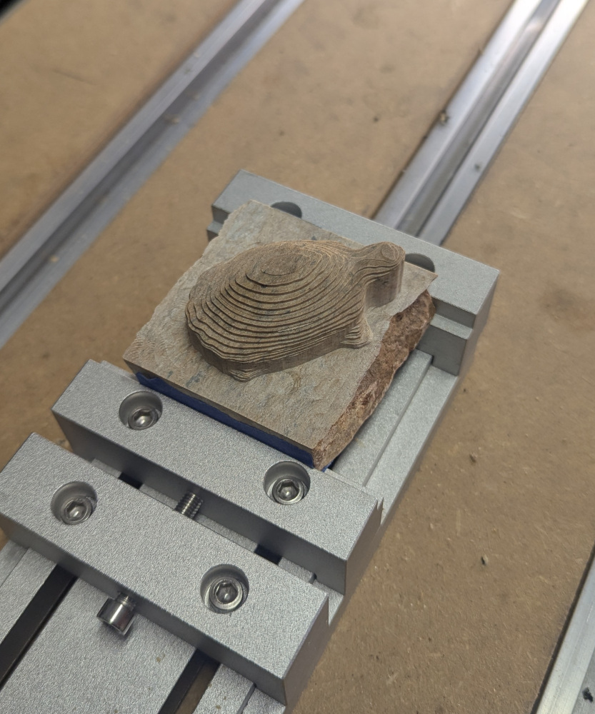
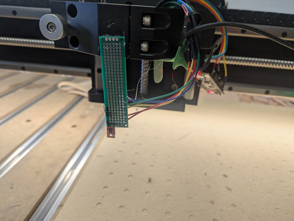
For the setup, I use a sparkfun magnetometer breakout board (MMC5983), hooked up to a regularly polling nucleo board that reported the data back to a computer over serial. Mounting it onto the Shapeoko allowed me to get it to a decent distance from motors and allowed me control the position with gcode.

As this is a quick project, I assigned the points to specific locations just based off of time in the scanned motion, and only calibrated by subtracting a background scan reading and applying the coordinate transforms as if the chip was exactly aligned with the machine coordinate systems.

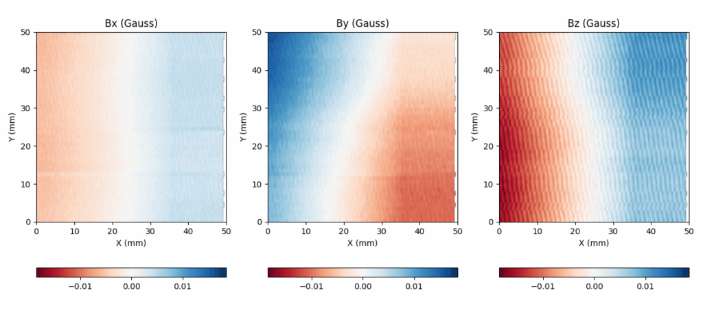
I imaged a cell phone and could see the fields of (presumably) speaker magnets at the top and bottom.

Field lines are visualized by integrating the motion of randomly placed test particles along the measured direction of the magnetic fields. I made these plots for a pair of small magnets, one vertically oriented and the horizontally.

I would like to redo this with a new board that has magnetic excitation coils (so the Earth’s field isn’t nessesary for imaging non-magnetized materials) and a design so the magnetometer could be moved almost flush with the sample to be images. I’m pretty sure one could image, if not inspect ENIG PCBs with this sort of technique.

Soapstone is a soft stone with a pleasing handfeel that’s often used for carving into small statues and molds. I’ve been wanting to CNC machine soapstone for some time, but have always avoided it on my mill because I don’t want the dust to damage the mechanics. The Shapeoko has a good dust boot, so I decided to go ahead with it.

For this, I used a 3D adaptive toolpath with a 1/4″ endmill followed by a contour toolpath with a tapered endmill with a 1mm radius ball at the end. My surface speeds were 12,500 IPM and feeds were 0.001 IPT.

I could not grip the stock hard enough in the vise until I tried adding a layer of painters tape along the bottom edge of the stock, which is a trick we occasionally used at my previous employer.

Unfortunately, it would take a heroic effort to machine the bottom of this, which I did for the Aluminum turtle to the side. On that one, I left the model attached by tabs while machining the bottom.

The dust boot was so effective that there was no dust left as evidence.

I am writing software to generate drag knife toolpaths from SVG files. Drag knife cuts do not exactly follow the toolpaths, and if this is to be corrected, a way of predicting the cut path given a toolpath is nessesary. I have done the pen and paper math to get a differential equation the cut should follow given a toolpath and compared that prediction to actual use of the drag knife, finding good agreement. In a future post I will show how to generate toolpaths that produce cuts that closely match the inputted desired cuts.

---

For a drag knife, the blade is offset backwards from the center of rotation and is freely rotating. Cutting is done at the blade offset \(r\) from the center of rotation, and at the angle of rotation \(\theta\) :

$$\vec{x}_{cut} = \vec{x}_{toolpath} + (r sin(\theta), r cos(\theta))$$

When the tool is engaged and the center of rotation moves, the tool angle changes such that the cutting point moves the shortest distance. We can find the actual equation describing \(\theta\) by writing out the quantity to minimize \((|\frac{d\vec{x}_{cut}}{dl}|)\), and minimizing it by taking a derivative and setting it equal to zero. This gives:

$$\frac{d\theta}{dl}=\frac{sin(\theta – \phi)}{r}$$

where \(l\) is the length along the path and \(\phi\) is the path angle. We see that smaller blade offsets will cause \(\theta\) to track \(\phi\) more tightly, however this is an ideal case and more force will be required with small \(r\) to overcome the rotational friction of the drag knife, stretching the material to be cut. As the blade is held at an \(\approx45^{\circ}\) angle from vertical and the material has nonzero thickness there is also some range of cutting radii and the material or blade needs to bend for any turn.

I use the following block of code to predict the simulated path by Euler integrating the angle and substituting it into the equation of cut position:

# Given a tool path, predict the actual cut path                                                                                                                                                                     
def simulate(path, theta0):

    lengths = np.concatenate(([0],np.cumsum(np.linalg.norm(np.diff(path, axis = 0), axis = 1))))
    path_interpolator = interp1d(lengths, path.T)

    # Blade angle                                                                                                                                                                                                    
    thetas = [theta0]
    # Path angle                                                                                                                                                                                                     
    phis = [0]

    toolpath_coords = [path_interpolator(0)]
    cut_coords = [path_interpolator(0) + BLADE_OFFSET_MM * np.array([np.sin(theta0), np.cos(theta0), 0])]

    n_points = int(POINTS_PER_MM * np.ceil(lengths[-1]))
    ls = np.linspace(0, lengths[-1], n_points)

    for i in range(1, n_points):
        ln = ls[i]
        lp = ls[i - 1]

        cn = path_interpolator(ln)
        toolpath_coords.append(cn)
        cp = path_interpolator(lp)

        # When not moving horizontally, just report previous movement direction                                                                                                                                      
        if (cn[0] - cp[0])**2 + (cn[1] - cp[1])**2 <= 1E-3:
            phis.append(phis[-1])
        else:
            phis.append(arctan2(cn[0] - cp[0], cn[1] - cp[1]))

        # Angle only updates when the tool is engaged at Z = 0                                                                                                                                                       
        if cn[2] == 0 and cp[2] == 0:
            thetas.append(thetas[-1] + (ln - lp) / BLADE_OFFSET_MM * np.sin(thetas[-1] - phis[-1]))
        else:
            thetas.append(thetas[-1])

        cut_coords.append(cn + BLADE_OFFSET_MM * np.array([np.sin(thetas[-1]), np.cos(thetas[-1]), 0]))

    thetas = np.array(thetas)
    phis = np.array(phis)
    toolpath_coords = np.array(toolpath_coords)
    cut_coords = np.array(cut_coords)

    return thetas, phis, toolpath_coords, cut_coords

For a real test case, I scanned through arcs of different total angle and turning radius. I made gcode following the paths, and then traced out the desired cut in blue ink, the simulated cut in red ink, and switched to the drag knife and followed the desired cut’s shape. Below is a photograph of the results, taken from the paper on a light box (it is easier to see in person). Agreement is pretty good, including the weird reversal shape that happens in the bottom right corner. Where the simulated path is hard to see corresponds to places where the cut followed the simulated toolpath almost exactly.